Idealized greenhouse model

The greenhouse effect can be illustrated with an idealized planet. This is a common "textbook model" ^[1]: the planet will have a constant surface temperature T_s and an atmosphere with constant temperature T_a. For diagrammatic clarity, a gap can be depicted between the atmosphere and the surface. Alternatively, T_s could be interpreted as a temperature representative of the surface and the lower atmosphere, and T_a could be interpreted as the temperature of the upper atmosphere. In order to justify that T_a and T_s remain constant over the planet, strong ocean and atmospheric currents can be imagined to provide plentiful lateral mixing. Furthermore, any daily or seasonal cycles in temperature are assumed to be insignificant.

The model will find the values of T_s and T_a that will allow the outgoing radiative power, escaping the top of the atmosphere, to be equal to the absorbed radiative power of sunlight. When applied to a planet like Earth, the outgoing radiation will be longwave and the sunlight will be shortwave. These two streams of radiation will have distinct emission and absorption characteristics. In the idealized model, we assume the atmosphere is completely transparent to sunlight. The planetary albedo α_P is the fraction of the incoming solar flux that is reflected back to space. The flux density of the incoming solar radiation is specified by the solar constant S₀. For application to planet Earth, appropriate values are S₀=1366 W m^-2 and α_P=0.30. Accounting for the fact that the surface area of a sphere is 4 times the area of its intercept (its shadow), the average incoming radiation is S₀/4.

For short wave radiation, the surface of the Earth is assumed to have an emissivity of 1. All incident shortwave radiation is completely absorbed. The surface emits a radiative flux density F according to the Stefan-Boltzmann law:

F = σT⁴

where σ is the Stefan-Boltzmann constant. A key to understanding the greenhouse effect is Kirchoff's law of thermal radiation. At any given wavelength the absorptivity of the atmosphere will be equal to the emissivity. Radiation from the surface could be in a slightly different portion of the infrared spectrum than the radiation emitted by the atmosphere. The model assumes that the average emissivity (absorptivity) is identical for either of these streams of infrared radiation, as they interact with the atmosphere. Thus, for longwave radiation, one symbol ε denotes both the emissivity and absorptivity of the atmosphere, for any stream of infrared radiation.

Idealized greenhouse model with an isothermal atmosphere. The blue arrows denote shortwave (solar) radiative flux density and the red arrow denotes longwave (terrestrial) radiative flux density. The radiation streams are shown with lateral displacement for clarity; they are collocated in the model. The atmosphere, which interacts only with the longwave radiation, is indicated by the layer within the dashed lines. A specific solution is depicted for ε=0.78 and α_p=0.3, representing Planet Earth. The numbers in the parentheses indicate the flux densities as a percent of S₀/4.

The equilibrium solution with ε=0.82. The increase by Δε=0.04 corresponds to doubling carbon dioxide and the associated positive feedback on water vapor.

The equilibrium solution with no greenhouse effect: ε=0

The infrared flux density out of the top of the atmosphere:

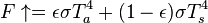
In the last term, ε represents the fraction of upward longwave radiation from the surface that is absorbed, the absorptivity of the atmosphere. In the first term on the right, ε is the emissivity of the atmosphere, the adjustment of the Stefan-Boltzmann law to account for the fact that the atmosphere is not optically thick. Thus ε plays the role of neatly blending, or averaging, the two streams of radiation in the calculation of the outward flux density.

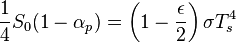
Zero net radiation leaving the top of the atmosphere requires:

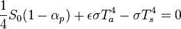
Zero net radiation entering the surface requires:

Energy equilibrium of the atmosphere can be either derived from the two above equilibrium conditions, or independently deduced:

Note the important factor of 2, resulting from the fact that the atmosphere radiates both upward and downward. Thus the ratio of T_a to T_s is independent of ε:

Thus T_a can be expressed in terms of T_s, and a solution is obtained for T_s in terms of the model input parameters:

or

The solution can also be expressed in terms of the effective emission temperature T_e, which is the temperature that characterizes the outgoing infrared flux density F, as if the radiator were a perfect radiator obeying F=σT_e⁴. This is easy to conceptualize in the context of the model. T_e is also the solution for T_s, for the case of ε=0, or no atmosphere:

With the definition of T_e:

For a perfect greenhouse, with no radiation escaping from the surface, or ε=1:

Using the parameters defined above to be appropriate for Earth,

For ε=1:

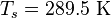
For ε=0.78,

.

This value of T_s happens to be close to a very widely quoted (but unattributed) 288 K claimed for the average global "surface temperature". ε=0.78 implies 22% of the surface radiation escapes directly to space, consistent with the statement of 15% to 30% escaping in the greenhouse effect.

The radiative forcing for doubling carbon dioxide is 3.71 W m^-2, in a simple parameterization. This is also the value endorsed by the IPCC. From the equation for ,

Using the values of T_s and T_a for ε=0.78 allows for = -3.71 W m^-2 with Δε=.019. Thus a change of ε from 0.78 to 0.80 is consistent with the radiative forcing from a doubling of carbon dioxide. For ε=0.80,

Thus this model predicts a global warming of ΔT_s = 1.2 K for a doubling of carbon dioxide. A typical prediction from a GCM is 3 K surface warming, primarily because the GCM allows for positive feedback, notably from increased water vapor. A simple surrogate for including this feedback process is to posit an additional increase of Δε=.02, for a total Δε=.04, to approximate the effect of the increase in water vapor that would be associated with an increase in temperature. This idealized model then predicts a global warming of ΔT_s = 2.4 K for a doubling of carbon dioxide, roughly consistent with the IPCC.